
THE SEQUENCE OF RETURN RISK CAN WORK BOTH FOR AND AGAINST YOU

When to seek it and when to avoid it. Discover why timing, not just performance, shapes your investment outcome.
Some investors believe that volatility and risk-adjusted returns are neither important nor relevant over long investment periods. This may be true if you invest a lump sum and don’t draw income from it. However, it is very different when you draw income from a lump-sum investment or make monthly contributions to an investment while accumulating wealth.
Getting this wrong can be very costly, and a different approach should be adopted to both benefit from and protect against the sequence of returns.
What is sequence risk?
Sequence risk relates to how and when poor investment returns can influence the long-term value of investments. It’s essential to recognise that sequence risk can impact long-term investment value either positively or negatively. The outcome depends on whether you are in the wealth accumulation (wealth building) phase or the wealth decumulation (income withdrawal) phase of your investing journey.
How are investments priced?
Most people invest in unit trusts, ETF’s or other investments that are priced per unit. The rands (or USD, Euro, GBP, etc.) that you invest in buy a certain number of units based on the unit price on that given day. Example: If you invest R5000 per month and the underlying unit price = R5.00, then you will buy 1 000 units of that investment. It stands to reason that the cheaper the units are, the more units you will get allocated. If the units referred to reduce to R2.50 per unit, then your R5000 will buy you 2 000 units. You will notice on your investment statements that you receive quarterly, reference is made to the number of units you own, the price per unit and the total investment value of the particular investment. (This is all very obvious, but stick with me…)
From the above, one can conclude that the cheaper the units are, the more units you will accumulate over time. This will be an advantage when there is a re-rating and the price per unit increases. It makes sense to buy cheaply. When you invest regularly (monthly), rand cost averaging will, in most cases, work in your favour, and price becomes less relevant.
The opposite is true when you draw income. In a similar manner to when you invest, the amount you need as income will require you to sell units. If the unit price reduces shortly after you invest, then you will have to sell more units than you bought to maintain your income. In the example above, if your R5 000 bought 1 000 units at R5.00 each and the price dropped to R2.50 per unit, you would have to sell 2 000 units to achieve the income. But you only bought 1 000 units – where will the other 1 000 units come from?
You will have to sell other investment units, which may lead to a capital loss. It makes sense to sell units when they have increased in value. It may also make sense to ringfence three years’ income and keep it in cash or a low volatility fund from where your regular income can be drawn. This will reduce the severity of sequence risk.
The age-old saying applies, buy low and sell high, especially when you need to draw income. The challenge is, how do you know when the price is low and when it is high?
In a perfect world, we would buy units very cheaply every month for 20 years and then see the unit prices increase significantly in value when we want to start drawing income from the investment. But we know that, unfortunately, it does not necessarily work like that. It does, however, teach us a valuable lesson: Don’t stop investing when prices drop. In fact, invest more!
Let’s take a look at a realistic example. I have borrowed the figures, some words and graphs from a recent article by Glacier – thank you, Glacier.
To illustrate some of the points above, we have randomly generated two fictitious 15-year investment portfolios with the following characteristics:
Portfolio A: 9% p.a. return (CPI+5% p.a. assuming inflation is 4% p.a.)
9% p.a. standard deviation (as for medium and high equity balanced funds)
Good early returns, followed by mediocre returns
Portfolio B: 9% p.a. return (CPI+5% p.a. assuming inflation is 4% p.a.)
9% p.a. standard deviation (as for medium and high equity balanced funds)
Poor early returns, followed by good returns.
The only difference between Portfolio A and Portfolio B is the sequence of their returns.
We also add a Target Return portfolio that grows consistently at 9% p.a. (with zero volatility)
Assumption:
A young investor takes out a new retirement annuity (RA)
The investor contributes R1 000 per month, which escalates by CPI+1% every year
We compare the investor’s RA balance after 15 years, assuming contributions were made to Portfolio A, Portfolio B and the Target Return portfolio.
The RA balance, over time under the three scenarios, is graphed as follows:
Figure 2: RA balance over time
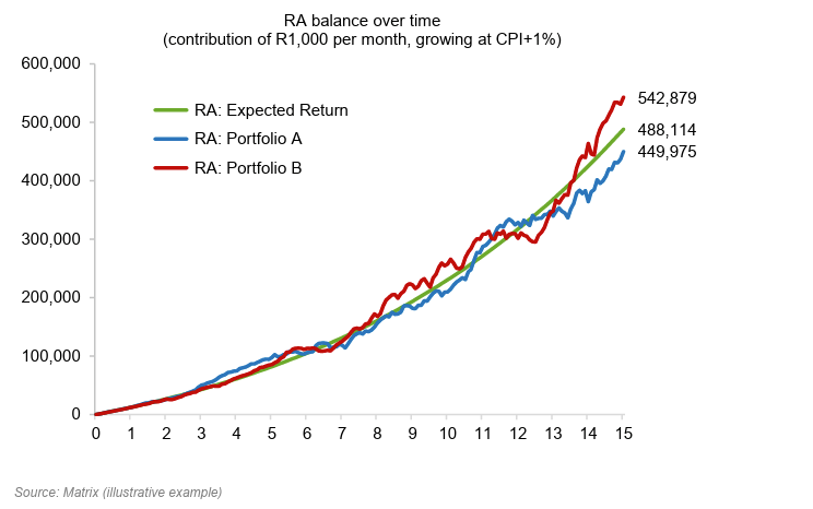
The RA linked to Portfolio B (poor early returns, then good returns later) performed better than the RA linked to Portfolio A (good early returns) and the Expected Return Portfolio.
The RA balance after 15 years in Portfolio B (R 542 879) was 21% higher than the RA balance in Portfolio A (R 449 975), even though both portfolios had exactly the same risk-return profiles.
Here we see how sequence risk (bad early returns) worked in favour of the RA investor.
The opposites of lump sum investments
When investing a lump sum, the average return determines the final amount, regardless of the sequence of returns. Whether poor returns occurred at the start or end of an investment period, it makes no difference. The average rules.
However, when you draw an income from a lump sum, typically like a living annuity, the sequence of returns becomes crucial. If you experience a couple of negative-return years at the start of your living annuity, it will be very difficult to recover, and the likelihood of forced reduced income in the future cannot be ruled out.
Below, we show a graph (typically as you will see on a fund’s MDD) that illustrates how a R100 lump sum at inception would have grown over 15 years in each portfolio.
Figure 1: Growth of R100 lump sum over 15 years
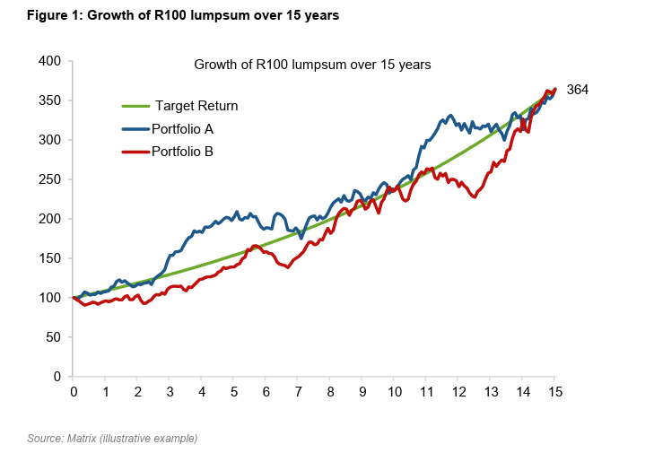
We note that both Portfolio A and Portfolio B have the same future value after 15 years.
Let’s now add an income drawn from the above lump sum, like a typical living annuity.
Consider the following example:
A new retiree purchases a living annuity (LA) with savings of R1000 000
The retiree chooses a 6% (R60 000 p.a.) initial drawdown rate, paid monthly.
The monthly pension increases by CPI+1% every year.
We now compare the retiree’s LA balance after 15 years, assuming withdrawals were made to Portfolio A, Portfolio B and the Target Return portfolio.
The LA balance over time, under the three scenarios, is graphed as follows:
Figure 3: Living annuity balance over time
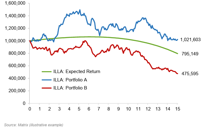
Here we note that:
The effect of sequence risk in the living annuity example is the opposite (and more dramatic) than in the RA example.
The LA linked to Portfolio B (poor initial returns) vastly underperforms the LA linked to Portfolio A (good initial returns).
The LA balance after 15 years linked to Portfolio A (R 1 021 603) was more than twice that of the LA balance linked to Portfolio B (R475 595), even though both portfolios had exactly the same risk-return profiles.
Now we see that sequence risk (bad early returns) had a dramatic negative impact on the LA retiree.
Equally important is to note the final value of the LA of portfolio A after 15 years. The value is slightly higher, but in real terms, lower than at the start, indicating that a return significantly greater than 9% will be necessary when drawing 6% income that escalates at 5% annually. Realistically, one can expect the value of the LA to decline in the future if all the assumed criteria remain unchanged.
Hopefully, this article will help some investors who struggle to understand basic investing principles. My apologies to those who found it oversimplified and boring, but thank you for reading the article.
Happy investing.
